#6: LaTeX
A quick introduction to LaTeX
What is LaTeX?
LaTeX, which is pronounced «Lah-tech» or «Lay-tech» (to rhyme with «blech» or «Bertolt Brecht»), is a document preparation system for high-quality typesetting. It is most often used for medium-to-large technical or scientific documents but it can be used for almost any form of publishing.
LaTeX is not a word processor! Instead, LaTeX encourages authors not to worry too much about the appearance of their documents but to concentrate on getting the right content.[1]
In many ways, LaTeX is similar to HTML where the author only specifies the structure of the document and leaves the styling to CSS.
When to and not to use LaTeX
LaTeX is the go-to tool if you’re
- writing a journal, article, book, presentation, or letter
- typesetting content with complex mathematical expressions, tables, or graphics
- writing large documents with chapters, citations, and cross-references
LaTeX is lightweight: it doesn’t come with a full-blown editor that lags when your document grows beyond a few hundred pages. Instead, it is built with resource optimisation in mind.
LaTeX is feature-rich: it is perfect for typesetting professional documents that involve complex content.
LaTeX is extensible: it works well with other tools to provide many of the features found in WYSIWYG editors. For example, version control is as simple as placing your LaTeX source files in a git repository.
However, LaTeX may not be best suited if you’re designing a poster, magazine cover, or similar document that requires precise and free visual control over page elements.
LaTeX with Overleaf
Overleaf is one of many LaTeX editors available to use. To quote their website, Overleaf is “The easy to use, online, collaborative LaTeX editor”.
While not FOSS software, Overleaf is free to access for all University of Birmingham students. To get started, head to https://www.overleaf.com/login and log in through your institution. We will discuss FOSS alternatives to Overleaf at the end of the lesson.

Let’s create a new project and explore what Overleaf has to offer.
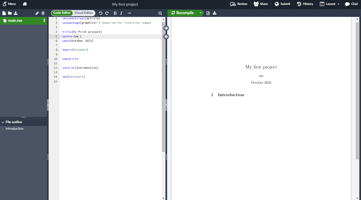
To the left are the project and file outline panels that list the files in a project and sections in the currently open document respectively. LaTeX projects are generally split across multiple .tex files, conventionally one for each section/chapter.
Next to them are the code editor and preview panels. The editor is where we will spend most of our time. Now is also a good time to enable auto compile from the “Recompile” drop-down to see previews as we go along.
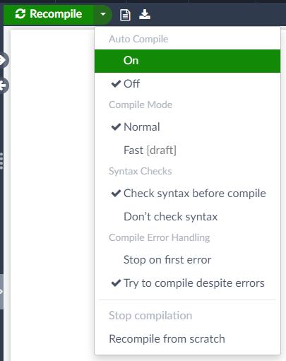
Now that we have a working LaTeX environment, let’s get started with typesetting!
The basics
The preamble
Our new document currently consists of the following mark-up:
\documentclass{article}
\usepackage{graphicx} % Required for inserting images

\title{My first project}
\author{me}
\date{October 2023}

\begin{document}

\maketitle

\section{Introduction}

\end{document}
The first part, i.e. the content between \documentclass... and ...\begin{document}, is called the preamble of the document. The preamble lets us define configuration options for the document and include any packages we may use.
Everything succeeding the preamble is the actual content of the document.
Document classes and packages
The \documentclass command defines the structure of the document’s layout, and takes an optional list of configuration options followed by the name of the document class as arguments. By default, Overleaf uses the article document class. Let’s switch to a landscape layout by specifying the landscape option, i.e., by using \documentclass[landscape]{article}.
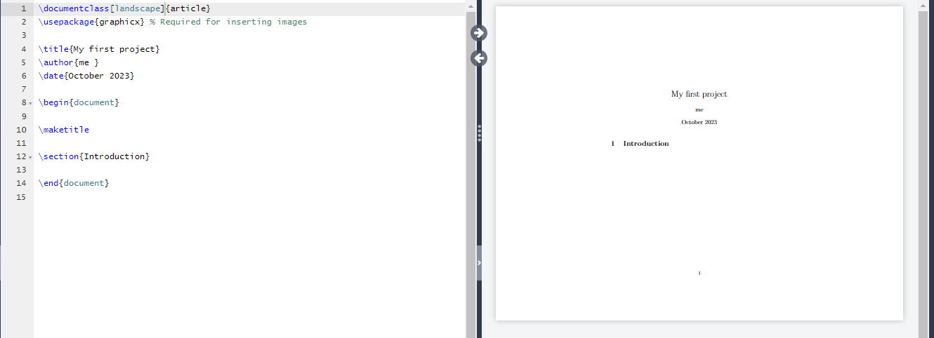
article, as the name suggests, is used to typeset articles and other basic content. As such, it lacks comprehensive configuration options and may not always be best suited for every document. Thankfully, there is a plethora of document classes for almost every need out there. An exhaustive list can be found on CTAN here. While we will use article for this lesson, below is an overview of a few popular document classes:
| Document class | Overview |
|---|---|
letter |
The standard LaTeX document class for writing letters |
beamer |
For typesetting presentations and slides |
acmart, IEEEtran |
For typesetting publications |
While writing your document, you will probably find that there are some areas where basic LaTeX cannot solve your problem. If you want to include graphics, colored text or source code from a file into your document, you need to enhance the capabilities of LaTeX. Such enhancements are called packages. Some packages come with the LaTeX base distribution. Others are provided separately. Modern TeX distributions come with a large number of packages pre-installed. The command to use a package is pretty simple: \usepackage[2].
For example, our document already includes the graphicx package using \usepackage{graphicx}.
A comprehensive list of packages can be found on CTAN. CTAN, the Comprehensive TeX Archive Network, is a set of sites that provide resources for TeX documents, e.g. packages, document classes, documentation, and more.
Typesetting basic stuff
Let’s add some content to the “Introduction” section of our new document.
\section{Introduction}
This is some \textbf{bold} and \textit{italicised} text.

Typesetting textual content is straightforward; you simply input the text to be displayed and the document class handles the typeface, positioning, and font size for you. Note how the \textbf and \textit commands are used to format text in bold and italics respectively.
Essentially, LaTeX allows you to focus on the content of your document and leave its appearance to the authors of the document class you’re using.
Typesetting more exciting stuff
Mathematical expressions
LaTeX only really starts to shine when used to typeset complex content that cannot be easily formatted in a WYSIWYG editor. A good example of this is mathematical expressions and equations. While this is not supported by LaTeX entirely out-of-the-box, mathematical statements can be typeset using the amsmath package with symbols from the amssymb package.
Below is a simple equation typeset inline with other text. Observe how the expression is enclosed in $ signs.
This is an equation of the form $x + y = z$

We can also typeset special characters using specific commands. For example,
$\alpha \rightarrow \sin(\Delta x)$
yields

Below are a few commonly used maths symbols:
| Category | Symbols | Commands |
|---|---|---|
| Relational operators | ≤ ≥ ≠ ⊂ | \leq, \geq, \neq, \subset |
| Vector operators | ⋅ × ∇ | \cdot, \times, \nabla |
| Greek letters | α β δ Δ | \alpha, \beta, \delta, \Delta |
| Miscellaneous | ∫ ∑ ∴ ∵ ∎ | \int, \sum, \therefore, \because, \QED |
A comprehensive list of symbols can be found here.
Fractions can be typeset using the \frac command which takes two arguments – the numerator and denominator expression.
$\frac{5x}{10} = \frac{x}{2}$

Equations
So far, we have only learned how to inline our maths expressions. Some use cases may require a full-width expression, say a theorem we might wish to introduce in our document. amsmath provides an equation environment that allows for this, which we use below to typeset the Pythagorean theorem.
\begin{equation}
    c^2 = b^2 + a^2
\end{equation}

Observe how LaTeX automatically numbers and centre-aligns the equation.
To typeset and align multiline equations, we use the align environment:
\begin{align}
    x^2 &= 49\\
    \therefore x &= \pm 7
\end{align}

The output can be thought of as a table where columns are demarcated by & and rows by \\. In other words, & denotes the end of a column and \\ denotes the end of a line. Using this information, amsmath typesets the equation such that all & are aligned one below the other. Observe how the two lines of differing length are aligned to the =symbol.
A handy tip to note is that automatic line numbering can be switched off by suffixing * to amsmath environments, e.g. \begin{align*} and \end{align*}. Alternatively, numbering can be turned off for specific lines by starting them with \nonumber. For example,
\begin{align}
    \nonumber x^2 &= 49\\
    \therefore x &= \pm 7
\end{align}

Code
As programmers, we often need to embed code snippets or entire programs in documents. There are LaTeX packages that, along with formatting code nicely, also provide syntax highlighting for a variety of languages. We will briefly cover two such packages: minted and listings.
Using minted
Code is embed inside a minted environment that allows for several customisations. For example, the following is some Java code that has been typeset with syntax highlighting and line numbers:
\begin{minted}[linenos]{java}
class Latex {
    public static final String message = "Typesetting code with LaTeX!";
}
\end{minted}

Similar to linenos, we can pass other options to the minted environment. Below is some python code highlighted using vim’s colour scheme and with a black background.
\begin{minted}[style=vim,bgcolor=black]{python}
def add(x, y):
    return x + y
\end{minted}

minted also allows for for embedding a single line of code:
\mint{js}|let someVariable = 5;|

A comprehensive list of what minted is capable of can be found here.
Using listings
listings is much more powerful and configurable than minted, but that comes with a steeper learning curve. Getting started is simple and basic code can be typeset almost identically to with minted
\begin{lstlisting}[language=Haskell]
    add :: Int -> Int -> Int
    add x y = x + y
\end{lstlisting}

The documentation for the package can be found here.
Images
Images are embedded using the graphicx package which Overleaf already imports for us. To add an image, we first upload the file to Overleaf.
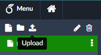
The image will show up in the file outline panel once uploaded successfully.
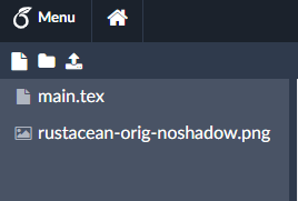
Next, we use the figure environment to embed the image in-line with other text.
\begin{figure}[ht]
    \centering
    \includegraphics[width=4cm]{rustacean-orig-noshadow.png}
    \caption{Rustacean}
    \label{fig:rustacean}
\end{figure}

There’s a lot happening here! Let’s break it down and analyse each bit.
- We pass the
htoptions to thefigureenvironment to place the image here (h), i.e. where the command appears in the document, and at the top of the page (t). An in-depth explanation of the positioning of floating elements in TeX can be found here. - The
\centeringcommand horizontally centres the image along the page. - The
\includegraphicscommand requires the image to display and, optionally, the dimensions of the displayed image. - The
\captioncommand displays a caption below the image. - The
\labelcommand attaches a non-visible label to the image that can be used to cite and cross-reference it from elsewhere in the document. We will cover this in more detail in a later section.
Trees and graphs
While there are several packages that support creating graphs, we will look at tikz, a powerful package to typeset all sorts of graphic elements.
We start off with the tikzpicture environment and the \node command to add a single node to the graph
\begin{tikzpicture}
    \node[{draw, circle}] (node1) {1};
\end{tikzpicture}

Here, we specify the stroke and shape of the node (draw, circle), give it a unique ID (node1), and typeset the content inside (1).
Similarly, it is possible to add multiple such nodes.
\begin{tikzpicture}[basic_node/.style = {draw, circle}]
    \node[basic_node] (node1) {1};
    \node[basic_node] (node2) {10};
    \node[basic_node] (node3) {100};
    \node[basic_node] (node4) {1000};
    \node[{draw}] (node5) {10000};
\end{tikzpicture}
Note how we’ve aliased the style of some nodes as basic_node for readability.

Uh oh! It seems all the nodes are rendered over one another. To fix this, we can specify a relative position for some nodes, as shown:
\begin{tikzpicture}[basic_node/.style = {draw, circle}]
    \node[basic_node] (node1) {1};
    \node[basic_node] (node2) [below left of = node1] {10};
    \node[basic_node] (node3) [below right of = node1] {100};
    \node[basic_node] (node4) [below left of = node2] {1000};
    \node[{draw}] (node5) [below left of = node3] {10000};
\end{tikzpicture}

That’s much better! We can now specify the edges between the nodes using the \draw command:
\begin{tikzpicture}[basic_node/.style = {draw, circle}]
    \node[basic_node] (node1) {1};
    \node[basic_node] (node2) [below left of = node1] {10};
    \node[basic_node] (node3) [below right of = node1] {100};
    \node[basic_node] (node4) [below left of = node2] {1000};
    \node[{draw}] (node5) [below left of = node3] {10000};

    \draw[->] (node1) -- (node2);
    \draw[->] (node1) -- (node3);
    \draw[->] (node2) -- (node4);
    \draw[->] (node3) -- (node5);
\end{tikzpicture}

Proof trees
There are several packages that support typesetting proof trees in the style of sequent calculus, and because this is not an unopinionated guide, we will look at one such package, ebproof.
Trees are typeset in prooftree environments and are mainly composed of hypotheses and inferences that are stacked up against each other.
Let’s typeset the following proof tree

\begin{prooftree}
\infer0[$[Id]$]{A \vdash A}
\infer1[$[\neg L]$]{\neg A, A \vdash B}

\infer0[$[Id]$]{B, A \vdash B}

\infer2[$[\vee L]$]{\neg A \vee B, A \vdash B}
\end{prooftree}
The proof tree can be broken down into several other subtrees, each of which is typeset separately and then combined to form the full tree. The \infer<N> set of commands define inferences that depend on N other inferences/hypotheses already in the stack. For example, \infer0 does not pop anything from the stack, but \infer2 pops two previously defined inferences from the stack.
The documentation for the ebproof package can be found here.
Integrating your work with Git
The structure of Overleaf projects is similar to that of a git repository, meaning we can clone, fork, pull from, and push to one just like any git repo. This enables you to work offline and sync your changes with Overleaf at a later time.
The option to sync with git can be found in the menu at the top left of the page.
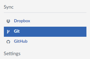
Clicking on it yields a link to a git repository that we can clone. Make sure to clone using authentication tokens, and generate a token if you don’t have one already.

If git prompts you for a username and password when cloning, enter git and your authentication token respectively.

We now have a git repository that we can work with. For a refresher on git, check out #5: Version Control and #2: Intermediate Shell + Git Basics. A more in-depth guide can be found here.
Citing and referencing content
Another area where LaTeX shines is when attributing and cross-referencing content.
The \ref command is used to reference labelled content from elsewhere in the document, i.e. content that was annotated with the \label command. Let’s go back to our embedded image from Typesetting more exciting stuff: Images that we labelled fig:rustacean.
Referencing it in the document is as easy as:
Figure~\ref{fig:rustacean} shows a picture of Ferris the crab.
To make the reference clickable, add the hyperref package to the preamble:
\usepackage[hidelinks]{hyperref}
Similarly, the \cite command works in conjunction with a .bib file to reference external content. As the name suggests .bib files consist of bibliography entries, like so:
@article{systems_programming_in_rust,
author = {Jung, Ralf and Jourdan, Jacques-Henri and Krebbers, Robbert and Dreyer, Derek},
title = {Safe Systems Programming in Rust},
year = {2021},
issue_date = {April 2021},
publisher = {Association for Computing Machinery},
address = {New York, NY, USA},
volume = {64},
number = {4},
issn = {0001-0782},
url = {https://doi.org/10.1145/3418295},
doi = {10.1145/3418295},
abstract = {The promise and the challenges of the first industry-supported language to master the trade-off between safety and control.},
journal = {Commun. ACM},
month = {mar},
pages = {144–152},
numpages = {9}
}
@inproceedings{comprehending_monads_wadler,
author = {Wadler, Philip},
title = {Comprehending Monads},
year = {1990},
isbn = {089791368X},
publisher = {Association for Computing Machinery},
address = {New York, NY, USA},
url = {https://doi.org/10.1145/91556.91592},
doi = {10.1145/91556.91592},
abstract = {Category theorists invented monads in the 1960's to concisely express certain aspects of universal algebra. Functional programmers invented list comprehensions in the 1970's to concisely express certain programs involving lists. This paper shows how list comprehensions may be generalised to an arbitrary monad, and how the resulting programming feature can concisely express in a pure functional language some programs that manipulate state, handle exceptions, parse text, or invoke continuations. A new solution to the old problem of destructive array update is also presented. No knowledge of category theory is assumed.},
booktitle = {Proceedings of the 1990 ACM Conference on LISP and Functional Programming},
pages = {61–78},
numpages = {18},
location = {Nice, France},
series = {LFP '90}
}
The .bib file above has two entries with additional metadata about the work being referenced. These were automatically generated by “cite” features offered by many journal websites. The two above were generated from their respective URLs at dl.acm.org.
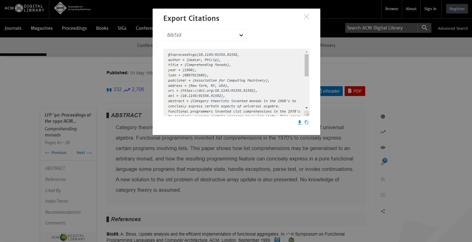
Before we can reference any of this work, we need to import the biblatex package in the preamble and add the .bib file (named references.bib) as a resource.
\usepackage{biblatex}
\addbibresource{references.bib}
We can now reference content like so:
Category theorists invented monads in the 1960's to concisely express certain aspects of universal algebra.~\cite{comprehending_monads_wadler}
And print the list of cited references, conventionally at the end of the document, like so:
\printbibliography
Note that depending on the document class you’re using, some or most of this work may already be taken care of for you.
Using LaTeX offline
Whether you’re working with a cloned local copy of your Overleaf project or are looking for FOSS alternatives, there are plenty of offline TeX engines to choose from.
If you’re on Windows, TeX Live and MikTeX are popular and time-tested TeX distributions. Alternatively, you could use the LaTeX Workshop extension on VSCode, which we will cover in a future session.
If you’re on MacOS, MacTeX and the homebrew package TeX Live are standard distributions to choose from.
If you’re on Linux, ask your package manager for a list of supported TeX engines.
Tectonic is a modern TeX engine written in Rust that is also worth checking out.
Whether on Overleaf or an offline TeX engine, we hope you continue exploring what LaTeX has to offer and are convinced to switch to it for all your document writing needs!
Licensed under CC BY-NC-SA.